Gaussian Process
Limbo relies on our C++-11 implementation of Gaussian processes (See Gaussian Process for a short introduction ) which can be useful by itself. This tutorial explains how to create and use a Gaussian Process (GP).
Data
We assume that our samples are in a vector called samples and that our observations are in a vector called observations. Please note that the type of both observations and samples is Eigen::VectorXd (in this example, they are 1-D vectors).
1 2 3 4 5 6 7 8 9 10 | // our data (1-D inputs, 1-D outputs)
std::vector<Eigen::VectorXd> samples;
std::vector<Eigen::VectorXd> observations;
size_t N = 8;
for (size_t i = 0; i < N; i++) {
Eigen::VectorXd s = tools::random_vector(1).array() * 4.0 - 2.0;
samples.push_back(s);
observations.push_back(tools::make_vector(std::cos(s(0))));
}
|
Basic usage
We first create a basic GP with an Exponential kernel (kernel::Exp<Params>) and a mean function equals to the mean of the observations (mean::Data<Params>). The Exp kernel needs a few parameters to be defined in a Params structure:
1 2 3 4 5 6 7 8 9 10 11 12 | struct Params {
struct kernel_exp {
BO_PARAM(double, sigma_sq, 1.0);
BO_PARAM(double, l, 0.2);
};
struct kernel : public defaults::kernel {
};
struct kernel_squared_exp_ard : public defaults::kernel_squared_exp_ard {
};
struct opt_rprop : public defaults::opt_rprop {
};
};
|
The type of the GP is defined by the following lines:
1 2 3 4 | // the type of the GP
using Kernel_t = kernel::Exp<Params>;
using Mean_t = mean::Data<Params>;
using GP_t = model::GP<Params, Kernel_t, Mean_t>;
|
To use the GP, we need :
- to instantiante a
GP_tobject - to call the method
compute().
1 2 3 4 5 | // 1-D inputs, 1-D outputs
GP_t gp(1, 1);
// compute the GP
gp.compute(samples, observations);
|
Here we assume that the noise is the same for all samples and that it is equal to 0.01.
Querying the GP can be achieved in two different ways:
gp.mu(v)andgp.sigma(v), which return the mean and the variance (sigma squared) for the input data pointvstd::tie(mu, sigma) = gp.query(v), which returns the mean and the variance at the same time.
The second approach is faster because some computations are the same for mu and sigma.
To visualize the predictions of the GP, we can query it for many points and record the predictions in a file:
1 2 3 4 5 6 7 8 9 10 11 12 | // write the predicted data in a file (e.g. to be plotted)
std::ofstream ofs("gp.dat");
for (int i = 0; i < 100; ++i) {
Eigen::VectorXd v = tools::make_vector(i / 100.0).array() * 4.0 - 2.0;
Eigen::VectorXd mu;
double sigma;
std::tie(mu, sigma) = gp.query(v);
// an alternative (slower) is to query mu and sigma separately:
// double mu = gp.mu(v)[0]; // mu() returns a 1-D vector
// double s2 = gp.sigma(v);
ofs << v.transpose() << " " << mu[0] << " " << sqrt(sigma) << std::endl;
}
|
Hyper-parameter optimization
Most kernel functions have some parameters. It is common in the GP literature to set them by maximizing the log-likelihood of the data knowing the model (see Gaussian Process for a description of this concept).
In limbo, only a subset of the kernel functions can have their hyper-parameters optimized. The most common one is SquaredExpARD (Squared Exponential with Automatic Relevance Determination).
A new GP type is defined as follows:
1 2 3 4 5 | // an alternative is to optimize the hyper-parameters
// in that case, we need a kernel with hyper-parameters that are designed to be optimized
using Kernel2_t = kernel::SquaredExpARD<Params>;
using Mean_t = mean::Data<Params>;
using GP2_t = model::GP<Params, Kernel2_t, Mean_t, model::gp::KernelLFOpt<Params>>;
|
It uses the default values for the parameters of SquaredExpARD:
1 2 3 4 | struct kernel : public defaults::kernel {
};
struct kernel_squared_exp_ard : public defaults::kernel_squared_exp_ard {
};
|
After calling the compute() method, the hyper-parameters can be optimized by calling the optimize_hyperparams() function. The GP does not need to be recomputed and we pass false for the last parameter in compute() as we do not need to compute the kernel matrix again (it will be recomputed in the hyper-parameters optimization).
1 2 3 | // do not forget to call the optimization!
gp_ard.compute(samples, observations, false);
gp_ard.optimize_hyperparams();
|
We can have a look at the difference between the two GPs:
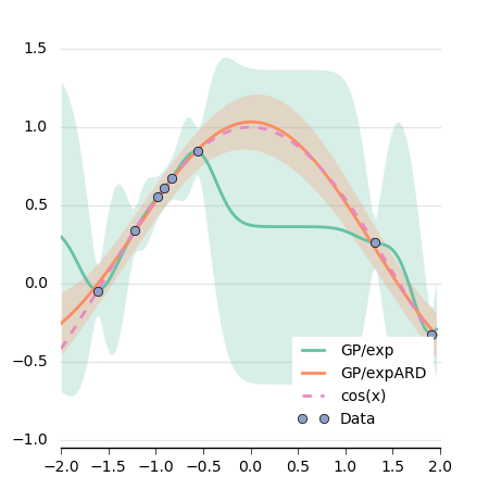
This plot is generated using matplotlib:
1 2 3 4 5 6 7 8 9 10 11 12 13 14 15 16 17 18 19 20 21 22 23 24 25 26 27 28 29 30 31 32 33 34 35 36 37 38 39 40 41 42 43 44 45 46 47 48 49 50 51 52 53 54 55 56 57 | import glob
from pylab import *
import brewer2mpl
# brewer2mpl.get_map args: set name set type number of colors
bmap = brewer2mpl.get_map('Set2', 'qualitative', 7)
colors = bmap.mpl_colors
params = {
'axes.labelsize': 8,
'text.fontsize': 8,
'legend.fontsize': 10,
'xtick.labelsize': 10,
'ytick.labelsize': 10,
'text.usetex': False,
'figure.figsize': [4.5, 4.5]
}
rcParams.update(params)
gp = np.loadtxt('gp.dat')
gp_ard = np.loadtxt('gp_ard.dat')
data = np.loadtxt('data.dat')
actual = []
for i in gp:
actual.append(math.cos(i[0]))
fig = figure() # no frame
ax = fig.add_subplot(111)
ax.fill_between(gp[:,0], gp[:,1] - gp[:,2], gp[:,1] + gp[:,2], alpha=0.25, linewidth=0, color=colors[0])
ax.fill_between(gp_ard[:,0], gp_ard[:,1] - gp_ard[:,2], gp_ard[:,1] + gp_ard[:,2], alpha=0.25, linewidth=0, color=colors[1])
ax.plot(gp[:,0], gp[:,1], linewidth=2, color=colors[0])
ax.plot(gp_ard[:,0], gp_ard[:,1], linewidth=2, color=colors[1])
ax.plot(gp[:,0], actual, linewidth=2, linestyle='--', color=colors[3])
ax.plot(data[:,0], data[:, 1], 'o', color=colors[2])
legend = ax.legend(["GP/exp", "GP/expARD", 'cos(x)', 'Data'], loc=8);
frame = legend.get_frame()
frame.set_facecolor('1.0')
frame.set_edgecolor('1.0')
ax.spines['top'].set_visible(False)
ax.spines['right'].set_visible(False)
ax.spines['left'].set_visible(False)
ax.get_xaxis().tick_bottom()
ax.get_yaxis().tick_left()
ax.tick_params(axis='x', direction='out')
ax.tick_params(axis='y', length=0)
for spine in ax.spines.values():
spine.set_position(('outward', 5))
ax.set_axisbelow(True)
ax.grid(axis='y', color="0.9", linestyle='-', linewidth=1)
fig.savefig('gp.png')
|
Here is the complete main.cpp file of this tutorial:
#include <fstream>
#include <limbo/kernel/exp.hpp>
#include <limbo/kernel/squared_exp_ard.hpp>
#include <limbo/mean/data.hpp>
#include <limbo/model/gp.hpp>
#include <limbo/model/gp/kernel_lf_opt.hpp>
#include <limbo/tools.hpp>
#include <limbo/tools/macros.hpp>
#include <limbo/serialize/text_archive.hpp>
// this tutorials shows how to use a Gaussian process for regression
using namespace limbo;
struct Params {
struct kernel_exp {
BO_PARAM(double, sigma_sq, 1.0);
BO_PARAM(double, l, 0.2);
};
struct kernel : public defaults::kernel {
};
struct kernel_squared_exp_ard : public defaults::kernel_squared_exp_ard {
};
struct opt_rprop : public defaults::opt_rprop {
};
};
int main(int argc, char** argv)
{
    // our data (1-D inputs, 1-D outputs)
    std::vector<Eigen::VectorXd> samples;
    std::vector<Eigen::VectorXd> observations;

    size_t N = 8;
    for (size_t i = 0; i < N; i++) {
        Eigen::VectorXd s = tools::random_vector(1).array() * 4.0 - 2.0;
        samples.push_back(s);
        observations.push_back(tools::make_vector(std::cos(s(0))));
    }
    // the type of the GP
    using Kernel_t = kernel::Exp<Params>;
    using Mean_t = mean::Data<Params>;
    using GP_t = model::GP<Params, Kernel_t, Mean_t>;
    // 1-D inputs, 1-D outputs
    GP_t gp(1, 1);

    // compute the GP
    gp.compute(samples, observations);
    // write the predicted data in a file (e.g. to be plotted)
    std::ofstream ofs("gp.dat");
    for (int i = 0; i < 100; ++i) {
        Eigen::VectorXd v = tools::make_vector(i / 100.0).array() * 4.0 - 2.0;
        Eigen::VectorXd mu;
        double sigma;
        std::tie(mu, sigma) = gp.query(v);
        // an alternative (slower) is to query mu and sigma separately:
        //  double mu = gp.mu(v)[0]; // mu() returns a 1-D vector
        //  double s2 = gp.sigma(v);
        ofs << v.transpose() << " " << mu[0] << " " << sqrt(sigma) << std::endl;
    }
    // an alternative is to optimize the hyper-parameters
    // in that case, we need a kernel with hyper-parameters that are designed to be optimized
    using Kernel2_t = kernel::SquaredExpARD<Params>;
    using Mean_t = mean::Data<Params>;
    using GP2_t = model::GP<Params, Kernel2_t, Mean_t, model::gp::KernelLFOpt<Params>>;
GP2_t gp_ard(1, 1);
    // do not forget to call the optimization!
    gp_ard.compute(samples, observations, false);
    gp_ard.optimize_hyperparams();
// write the predicted data in a file (e.g. to be plotted)
std::ofstream ofs_ard("gp_ard.dat");
for (int i = 0; i < 100; ++i) {
Eigen::VectorXd v = tools::make_vector(i / 100.0).array() * 4.0 - 2.0;
Eigen::VectorXd mu;
double sigma;
std::tie(mu, sigma) = gp_ard.query(v);
ofs_ard << v.transpose() << " " << mu[0] << " " << sqrt(sigma) << std::endl;
}
// write the data to a file (useful for plotting)
std::ofstream ofs_data("data.dat");
for (size_t i = 0; i < samples.size(); ++i)
ofs_data << samples[i].transpose() << " " << observations[i].transpose() << std::endl;
// Sometimes is useful to save an optimized GP
gp_ard.save<serialize::TextArchive>("myGP");
// Later we can load -- we need to make sure that the type is identical to the one saved
gp_ard.load<serialize::TextArchive>("myGP");
return 0;
}
Saving and Loading
We can also save our optimized GP model:
1 2 | // Sometimes is useful to save an optimized GP
gp_ard.save<serialize::TextArchive>("myGP");
|
This will create a directory called myGP with several files (the GP data, kernel hyperparameters etc.). If we want a binary format (i.e., more compact), we can replace the TextArchive by BinaryArchive.
To the load a saved model, we can do the following:
1 2 | // Later we can load -- we need to make sure that the type is identical to the one saved
gp_ard.load<serialize::TextArchive>("myGP");
|
Note that we need to have the same kernel and mean function (i.e., the same GP type) as the one used for saving.